Big O notation can be different to those unfamiliar with the concept. So to begin here’s a little road map of a few hot topics that I find frequently when the subject is spoken about.

1. What is Big O (and which one are we talking about?)

2. Why Big O?

3. Examples of Big O in the Not-So Wild: Datastructures and Sorts

What is Big O?

Big O describes the efficiency of an algorithm. Specifically it’s used to describe both the efficiency in time (Big O Time) and memory use (Big O Space) of an algorithm. If you’re non-technical, know that an algorithm is just a process of operations designed to solve a problem.

Sorting through an array? You just used an algorithm!

Selecting an instance from a database? Algorithm!

Finding the middle point for you and a friend to meet? Algoooo

Now there are three different types of Big O used in academia (Big O, Big Omega, and Big Theta) to describe runtime. Big O corresponds to the upper bound in a graph, Big Omega the lower bound, and Big Theta the tight bound.

These concepts shouldn’t be confused with best, worst, and expected case scenarios; each O notation can be used to describe each scenario. That being said, the Big notation used in programming, Big O (which in academia is closer to Big Theta) i.e. the tight bound for a function will be focused on.

Big O describes the rate of increase (in memory i.e. space or time) as “n”, your input, goes up. If your “n” is equal to an array, and you have to iterate through that array, you’re going to do that in Big O(n) time, where n is the number of elements in the input array. If you have an array that you’re grabbing an element from a specific index, that will take Big O(1) time, as it is done in 1 step no matter how large the array is.

Say we needed to run through an array twice,  does it take Big O(2n) time? No, we’d still say that it takes Big O(n) time. When we describe Big O we don’t use constants. A function that runs in Big O(n) we say will equal a function that runs in Big O(2n) because for different values of “n” those can be equal. So never use constants when you’re describing a runtime!

Why Big O?

We use Big O to find the time and memory that will be required to run a function. But what does that really mean and why care?

Well let’s say that you just got a job with a dating company with 200 members and this job pays you to pick matches among those people. 100 guys and 100 girls. Profiles are in an array and each user can match with either sex. Well let’s say that the company doesn’t allow you to skip users, and users don’t get removed from the dating pool when they’re matched with someone else.

So you begin manually. You’re presented with one person’s picture and then you go through each of the 200 (including the same person’s picture) to create matches. Until you go through each potential partner, then you start on the second partner…ad nauseum. It takes about 5 seconds per picture and since you don’t get your check until you finish, it takes 55.55 hours! That’s because the run time for the function is Big O(n^2). For each person on the site, you have to go through the every individual again.

What’s more efficent? Just about anything. You could seek to limit the number of users that an individual get’s access to by grouping and matching based upon a set of preferences. Or stop once a user has a certain number of matches.

But what about Big O space? Well let’s use those that examples again. In the situation you’ll have to use some sort of data structure to store your matches for a person. Let’s say you use another array. That means that each person will need to have their own for their matches. That means you’re about to build out 200 array’s of up to 200 people each…now that doesn’t take much time to add to as pushing to an array takes Big O(1) time. But now you have n users each with an n sized array that’s n^2 spaced. The problems you face when you start to consider the implications of algorithms speed and space constraints will often be give and take. It’s always about finding the solution with the best pro to con ratio for your situation.

Examples of Big O in the Not-So Wild: Datastructures and Sorts

Big O comes in the most handy when thinking about data structures and sorting algorithms. We’re going to be going over these in the next several posts in this series, but for now, we’ll just begin by describing them and their various methods and runtimes.

First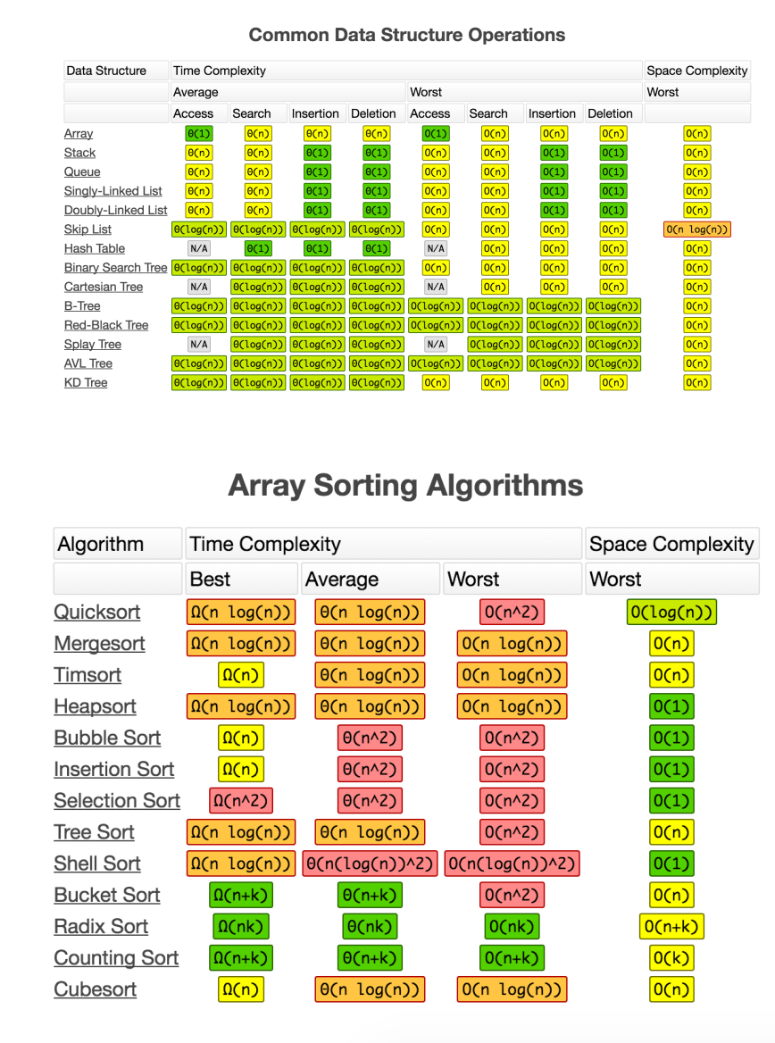 

Datastructures :

Array:  The array is a foundational data structure. It’s unique capability that makes it invaluable, is it’s O(1) time for access and insertion. If you know the position of an element, you can immediately get access to it. Array’s in many languages are often used to create other datastructures like stacks, queues, and hash tables.

Stack: A stack is a datastructure that is peculiar in the fact that it works like a LIFO, Last in First Out, array. The latest addition to the stack, would be accessed first, while the others can only be accessed by popping out the previous item one before itself. Think of stacks like the toddler game the tower of babel. Generally Stacks will use functions like push(item), pop(), peek(), and search(item). These methods take O(1), O(1), O(1), and O(n) time respectively. Stacks can be used to implement queues and are often used in DFS algorithms.

Queue: A queue is a datastructure that is peculiar in the fact that it is a FIFO, First in First Out, array. Meaning that the oldest item in the queue, is the first out of the Queue. Like a Stack, Queue can only be searched by going through each element. Think about a Queue like you would any line you’ve ever been in. Queues generally will use functions like unshift(), push(item), peek() (to view the bottom element), and search(item). These methods take O(1), O(1), O(1), and O(n) time respectively. Queues are often used in BFS algorithms.

Singly-Linked List: A Singly-Linked List (SLL) is a datastructure that is peculiar in the fact that each node is connected only to the next node, with the exception of the last node. the the oldest addition to the SLL, the Head/root, is only one that a user has direct accessiblity to, much like a queue. SSL’s can only be searched by going through each node’s ’next’ attribute that points to the following node. In a similar way to queue, adding and removing from/to the beginning of a SSL can be done in O(1) time, while adding/removing/searching to any other point would take O(n) time.

Hash Table: A Hash Table is a datastructure that is peculiar in the fact that it’s essentially an array with a plan. It contains buckets filled with key-value pairs that allows you to access any element in O(1) time and add or delete any item in O(1) time. A hash is stores its key value pairs via a hashing function that uses the input items key to create a hash and via another algorithm will calculate an index that points to a particular bucket in the array. Hash tables can be remarkably efficient with the correct hashing implementation. Hashes are a critical datastructures that’s also often used in conjunction with other more advanced datastructures.

Trees: A tree is a datastructure, that are similar to SSL’s in the way that they’re made up of nodes that connect to other nodes. Unlike SSL’s though, these nodes have links to both their parent and children nodes. Nodes that don’t have children are called leaf nodes. The first node is called the root. There are several different sorts of Trees, from trees that only accept 2 children (Binary trees and Binary Search Trees), to some that only offer a single character of information (Tries). Tree’s are used to connect points of information that relate to one another, and can be used with a variety of data structures. Sorted trees often have some of the best Big O search capabilities at O(n log(n)) as they can follow branches based off of simple conditionals.

Sorting Algorithms:

Quick Sort:  The Quick Sort algorithm works by finding a pivot point, and then sorting the two resulting arrays around said pivot point. The act of finding this pivot point will generally sort the array into a higher side, and a lower side. Depending on the size of array, this pivot point will be found recursively on each minor array. The act of finding this pivot point is an algorithm in itself, and several different of these have made their way into modern use with the Hoare partition being the most efficient. With sorts you do have to worry about the average AND worst case scenario of time it will take, as it can be something to worry about because who knows how your data will be positioned? It’s average time is O(n log(n)), but it can be as bad as O(n^2) in the right conditions. The quicksort is the sort of choice for most JS sorting alg’s.

By en:User:RolandH, CC BY-SA 3.0, https://commons.wikimedia.org/w/index.php?curid=1965827

Merge Sort: The merge sort works on the “Divide and Conquer” theory. It divides lists into sublists, then sorts those sublists, it then combines, and repeats the division as necessary. The final sublist becomes the ultimate sorted list. It is a remarkably resourceful sort whose expected and worst case sorts are both O(n log(n)).

By Swfung8 - Own work, CC BY-SA 3.0, https://commons.wikimedia.org/w/index.php?curid=14961648

Bubble Sort: The bubble sort works by “bubbling up” higher values with lower values. It’s a commonly used sorting tactic for trees and lists, where you can only access one value at a time. In order to do so, you must iterate through the array potentially n^2 times, making it a very time costly sort to do, with an average of O(n^2) time.

By Swfung8 - Own work, CC BY-SA 3.0, https://commons.wikimedia.org/w/index.php?curid=14953478

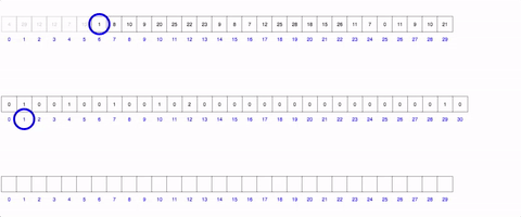
Counting Sort: The counting sort is personally my favorite sort. Unfortunately it does have certain parameters that your data may or may not have: each value in the data must be an integer, you must know the max integer within it, and all the values must be positive. The graphic below shows it (decently). it relies on the creation of a new array from the size of the max value. You then iterate through the unsorted array, and every time you find a new number add 1 to the index of the range array to the index of that number. So if you have an array with 3 1’s,  rangeArray[1] will equal 3! This addition to the rangeArray takes O(1) time due to Array’s O(1) access time! You then (can) create a third final array which as you go through each index, you check the rangeArray and add each number the corresponding amount of times that it has in its “counter”. This array in itself feels like a beautiful hack of the datastrucutres O(1) access time and can be done consistently in O(n+k) time and space.

True learning happens in the off hours when you actively apply the tools you’ve taught yourself about. These tools above are just a small subset in computer science that can help you in a variety of ways. Try and use them.